Algorithms

Complexity

Amortized Analysis

Amortized analysis is a method for analyzing a given algorithm's complexity, or how much of a resource, especially time or memory, it takes to execute.

Amortized analysis requires knowledge of which series of operations are possible. This is most commonly the case with data structures, which have state that persists between operations. The basic idea is that a worst-case operation can alter the state in such a way that the worst case cannot occur again for a long time, thus "amortizing" its cost.

There are generally three methods for performing amortized analysis: the aggregate method, the accounting method, and the potential method. All of these give correct answers; the choice of which to use depends on which is most convenient for a particular situation.

• Aggregate analysis determines the upper bound \(\mathcal{T}(n)\) on the total cost of a sequence of \(n\) operations, then calculates the amortized cost to be \(\mathcal{T}(n) / n\).
• The accounting method is a form of aggregate analysis which assigns to each operation an amortized cost which may differ from its actual cost. Early operations have an amortized cost higher than their actual cost, which accumulates a saved "credit" that pays for later operations having an amortized cost lower than their actual cost. Because the credit begins at zero, the actual cost of a sequence of operations equals the amortized cost minus the accumulated credit. Because the credit is required to be non-negative, the amortized cost is an upper bound on the actual cost. Usually, many short-running operations accumulate such credit in small increments, while rare long-running operations decrease it drastically.
• The potential method is a form of the accounting method where the saved credit is computed as a function (the "potential") of the state of the data structure. The amortized cost is the immediate cost plus the change in potential.

Array ExampleFIFO Queue Example

Consider a dynamic array that grows in size as more elements are added to it, such as ArrayList in Java or std::vector in C++. If we started out with a dynamic array of size 4, we could push 4 elements onto it, and each operation would take constant time. Yet pushing a fifth element onto that array would take longer as the array would have to create a new array of double the current size (8), copy the old elements onto the new array, and then add the new element. The next three push operations would similarly take constant time, and then the subsequent addition would require another slow doubling of the array size.

In general, for an arbitrary number \(n\) of pushes to an array of any initial size, the times for steps that double the array add in a geometric series to \(\mathcal{O}(n)\), while the constant times for each remaining push also add to \(\mathcal{O}(n)\). Therefore the average time per push operation is \(\mathcal{O}(n)/n = \mathcal{O}(1)\).

class Queue:
    # Initialize the queue with two empty lists
    def __init__(self):
        self.input = []  # Stores elements that are enqueued
        self.output = []  # Stores elements that are dequeued

    def enqueue(self, element):
        self.input.append(element)  # Append the element to the input list

    def dequeue(self):
        if not self.output:  # If the output list is empty
            # Transfer all elements from the input list to the output list, reversing the order
            while self.input:  # While the input list is not empty
                self.output.append(
                    self.input.pop()
                )  # Pop the last element from the input list and append it to the output list

        return self.output.pop()  # Pop and return the last element from the output list

The enqueue operation just pushes an element onto the input array; this operation does not depend on the lengths of either input or output and therefore runs in constant time.

However the dequeue operation is more complicated. If the output array already has some elements in it, then dequeue runs in constant time; otherwise, dequeue takes \(\mathcal{O}(n)\) time to add all the elements onto the output array from the input array, where \(n\) is the current length of the input array. After copying \(n\) elements from input, we can perform \(n\) dequeue operations, each taking constant time, before the output array is empty again. Thus, we can perform a sequence of \(n\) dequeue operations in only \(\mathcal{O}(n)\) time, which implies that the amortized time of each dequeue operation is \(\mathcal{O}(1)\).

Alternatively, we can charge the cost of copying any item from the input array to the output array to the earlier enqueue operation for that item. This charging scheme doubles the amortized time for enqueue but reduces the amortized time for dequeue to ⁠\(\mathcal{O}(1)\).

Binary Search

Find insert position

IntuitionAlgorithm

Binary search is a search algorithm that finds the position of a target value within a sorted array.

Usually, within binary search, we compare the target value to the middle element of the array at each iteration.

• If the target value is equal to the middle element, the job is done.
• If the target value is less than the middle element, continue to search on the left.
• If the target value is greater than the middle element, continue to search on the right.
• If the target value is not found, the loop will be stopped at the moment when right < left and nums[right] < target < nums[left]. Hence, the proper position to insert the target is at the index left.

1. Starting from left = 0 and right = n - 1, we then move either of the pointers according to various situations:
2. While left <= right:
   1. The pivot index is the one in the middle: pivot = (left + right) / 2. The pivot also divides the original array into two subarrays.
   2. If the target value is equal to the pivot element: target == nums[pivot], we're done.
   3. If the target value is less than the pivot element target < nums[pivot], continue to search on the left subarray by moving the right pointer right = pivot - 1.
   4. If the target value is greater than the pivot element target > nums[pivot], continue to search on the right subarray by moving the left pointer left = pivot + 1.
3. If not stopped already, return left.

def searchInsert(nums: List[int], target: int) -> int:
    L = 0
    R = len(nums) - 1
    while L <= R:
        PVT = (L + R) // 2
        if nums[PVT] == target:
            return PVT
        elif target < nums[PVT]:
            R = PVT - 1
        else:
            L = PVT + 1
    return L

Search a 2D Matrix

You are given an m x n integer matrix matrix with the following two properties: Each row is sorted in non-decreasing order. The first integer of each row is greater than the last integer of the previous row. Given an integer target, return true if target is in matrix or false otherwise.

IntuitionComplexityClassic MethodRecursive Method

Since each row is sorted and the first element of each row is greater than the last of the previous, we can treat the matrix like a flattened sorted array and apply binary search.

Time Complexity: \(\mathcal{O}(\log(m \star n))\) binary search over all elements Space Complexity: \(\mathcal{O}(1)\) constant space used

def searchMatrix(matrix: List[List[int]], target: int) -> bool:
    rows, cols = len(matrix), len(matrix[0])
    start, end = 0, rows * cols - 1

    while start <= end:
        mid = (start + end) // 2
        row, col = mid // cols, mid % cols
        current = matrix[row][col]

        if current == target:
            return True

        if current < target:
            start = mid + 1
        else:
            end = mid - 1

    return False

def searchMatrix(matrix: List[List[int]], target: int) -> bool:
    idx = len(matrix) // 2
    if len(matrix) == 0: return False
    start, end = matrix[idx][0], matrix[idx][-1]
    if target in matrix[idx]:
        return True
    elif target < start:
        return self.searchMatrix(matrix=matrix[:idx], target=target)
    elif target > end:
        return self.searchMatrix(matrix=matrix[idx+1:], target=target)
    else:
        return False

Peak detection

A peak element is an element that is strictly greater than its neighbors. Given a 0-indexed integer array nums, find a peak element, and return its index. If the array contains multiple peaks, return the index to any of the peaks.

Since we only need one peak, and the array's values are distinct enough, we can leverage binary search rather than scanning linearly.

Intuition

1. Use two pointers, left and right, to bound the search space.
2. At each step, calculate mid.
3. If nums[mid] > nums[mid + 1], the peak is to the left, including mid.
4. Otherwise, the peak is to the right.
5. The loop stops when left == right, which will be a peak.

This efficient binary search approach guarantees finding a peak in logarithmic time

ComplexityImplementation

Time Complexity: \(\mathcal{O}(\log(n))\) binary search Space Complexity: \(\mathcal{O}(1)\) constant space used

def findPeakElement(nums: List[int]) -> int:
    start, end = 0, len(nums) - 1
    while start != end:
        mid = (start + end) // 2
        if nums[mid] > nums[mid+1]:
            # peak is to the left
            end = mid
        else:
            # peak is to the right
            start = mid + 1
    return start

Sliding Window

Minimum Size Subarray Sum

Given an array of positive integers nums and a positive integer target, return the minimal length of a subarray whose sum is greater than or equal to target. If there is no such subarray, return 0 instead.

IntuitionAlgorithm

Pseudocode

function fn(arr):
    left = 0
    for (int right = 0; right < arr.length; right++):
        Do some logic to "add" element at arr[right] to window

        while WINDOW_IS_INVALID:
            Do some logic to "remove" element at arr[left] from window
            left++

        Do some logic to update the answer

def minSubArrayLen(target: int, nums: List[int]) -> int:
    left, right, run_sum = 0, 0, 0
    res = float('inf')
    for right in range(len(nums)):
        run_sum += nums[right]
        while run_sum >= target:
            res = min(res, right - left + 1)
            run_sum -= nums[left]
            left += 1
    return res if res != float('inf') else 0

Backtracking

Template

def backtrack(candidate):
    if find_solution(candidate):
        output(candidate)
        return

    # iterate all possible candidates.
    for next_candidate in list_of_candidates:
        if is_valid(next_candidate):
            # try this partial candidate solution
            place(next_candidate)
            # given the candidate, explore further.
            backtrack(next_candidate)
            # backtrack
            remove(next_candidate)

Kadane's Algorithm

n computer science, the maximum sum subarray problem, also known as the maximum segment sum problem, is the task of finding a contiguous subarray with the largest sum, within a given one-dimensional array A[1...n] of numbers. It can be solved in \(\mathcal{O}(n)\) time and \(\mathcal{O}(1)\) space. Kadane' Algorithm is an algorithm to solve it.

IntuitionAlgorithm

1. Initialize 2 integer variables. Set both of them equal to the first value in the array.
   • current_sum will keep the running count of the current subarray we are focusing on.
   • best_sum will be our final return value. Continuously update it whenever we find a bigger subarray.
2. Iterate through the array, starting with the 2nd element (as we used the first element to initialize our variables). For each number, add it to the current_sum we are building. If current_sum becomes negative, we know it isn't worth keeping, so throw it away. Remember to update best_sum every time we find a new maximum.
3. Return best_sum

def max_subarray(numbers):
    """Find the largest sum of any contiguous subarray."""
    best_sum = float('-inf')
    current_sum = 0
    for x in numbers:
        # clever way to update current_sum when encountering negative numbers
        current_sum = max(x, current_sum + x)
        best_sum = max(best_sum, current_sum)
    return best_sum

Sum Problems

Two SumTwo Sum IIThree SumThree Sum (optimized)

Given an array of integers nums and an integer target, return indices of the two numbers such that they add up to target.

 def twoSum(nums: List[int], target: int) -> List[int]:
    mapping = {}
    for i, n in enumerate(nums):
        remainder = target - n
        if remainder in mapping:
            return [mapping[remainder], i]
        else:
            mapping[n] = i

Given a 1-indexed array of integers numbers that is already sorted in non-decreasing order, find two numbers such that they add up to a specific target number. Let these two numbers be numbers[index1] and numbers[index2] where 1 <= index1 < index2 <= numbers.length. Return the indices of the two numbers, index1 and index2, added by one as an integer array [index1, index2] of length 2.

def twoSum(numbers: List[int], target: int) -> List[int]:
    p1, p2 = 0, len(numbers) - 1

    while True:
        candidate = numbers[p1] + numbers[p2]
        if candidate == target:
            break
        elif candidate < target:
            p1 += 1
        elif candidate > target:
            p2 -= 1
    return [p1+1, p2+1]

Given an integer array nums, return all the triplets [nums[i], nums[j], nums[k]] such that i != j, i != k, and j != k, and nums[i] + nums[j] + nums[k] == 0. Notice that the solution set must not contain duplicate triplets.

The intuition is to reduce the 3 sum problem to a two sum, by fixing one pointer and thus reduce the search space.

def threeSum(nums: List[int]) -> List[List[int]]:
    target = 0
    nums = sorted(nums)
    solutions = set()
    prevp1 = None

    for p1 in range(0, len(nums)-3+1):
        # if we have seen this value already, skip it
        if p1 == prevp1:
            continue
        p1val = nums[p1]
        remnums = nums[p1+1:]
        p2, p3 = 0, len(remnums) - 1
        if p2 == p3:
            continue
        while True:
            if p3 <= p2:
                break
            candidate = p1val + remnums[p2] + remnums[p3]
            if candidate == target:
                solutions.add((p1val, remnums[p2], remnums[p3]))
                p2 += 1
                p3 -= 1
            elif candidate < target:
                p2 += 1
            elif candidate > target:
                p3 -= 1
        prevp1 = p1
    return list(solutions)

def threeSum(nums: List[int]) -> List[List[int]]:
    # Init variables that will hold the response and duplicates
    response, duplicates = set(), set()
    # Init lookup for already seen complements
    seen = {}
    # Iterate through the array so we can anchor the 3sum problem and reduce it to a 2sum.
    for i, v1 in enumerate(nums):
        # Check if value has already been handled - we do not want duplicates.
        if v1 not in duplicates:
            # Make sure we will never touch this value again in the future.
            duplicates.add(v1)
            # For the remainder of the nums list, iterate with the next value
            for j, v2 in enumerate(nums[i+1:]):
                # Calculate the complement
                # this is the final piece that is missing to get to the target 0
                complement = - v1 - v2
                if complement in seen and seen[complement] == i:
                    response.add(tuple(sorted((v1, v2, complement))))
                # This allows us to use the nums[j] as a complement for nums[i]
                seen[v2] = i
    return [list(triplet) for triplet in response]

Dynamic Programming

Template

1. Start with the recursive backtracking solution
2. Optimize by using a memoization table (top-down2 dynamic programming)
3. Remove the need for recursion (bottom-up dynamic programming)
4. Apply final tricks to reduce the time / memory complexity

Staircase Costs

ApproachNaïve Approach (slow)Efficient (fast)

Similar to the staircase problem mentioned in Fibonacci.

You are given an integer array cost where cost[i] is the cost of ith step on a staircase. Once you pay the cost, you can either climb one or two steps. You can either start from the step with index 0, or the step with index 1. Return the minimum cost to reach the top of the floor.

Basically a bruteforce approach.

• Time: \(\mathcal{O}(2^n)\)
• Space: \(\mathcal{O}(1)\) constant space

def minCostClimbingStairs(cost: List[int]) -> int:
    def simulate(c, i):
        if i + 1 == len(cost) or i + 2 == len(cost):
            return c[0]
        else:
            return c[0] + min(simulate(c[1:], i + 1), simulate(c[2:], i + 2))
    return min(simulate(cost, 0), simulate(cost[1:], 1))

Add up all costs in one go.

• Time: \(\mathcal{O}(N)\)
• Space: \(\mathcal{O}(1)\) constant space

def minCostClimbingStairs(cost: List[int]) -> int:
    n = len(cost)
    for i in range(2, n):
        cost[i] += min(cost[i-1], cost[i-2])
    return min(cost[n-1], cost[n-2])

Sorting

Countingsort

IntuitionBenefitsDrawbacksSample ImplementationPractical Example: H-Index

• Counts the values instead of compares them.
• The helper array is used to calculate the position.

• Complexity is \(\mathcal{O}(n + k)\) (aka linear) compared to other sorting algorithms who are \(\mathcal{O}(n \log n)\).
• Does not compare values but count them in a seperate array with \(k\) values.

• Is only suited for small variatiation of values compared the amount of values. E.g. sort all inhabitants of switzerland by age.

def counting_sort(arr):
    # 1. Find the maximum element to determine the range
    max_val = max(arr)

    # 2. Initialize count array with zeros
    count = [0] * (max_val + 1)

    # 3. Store the count of each element
    for num in arr:
        # Basic check for non-negative assumption
        if num < 0:
            raise ValueError("Counting sort requires non-negative integers.")
        count[num] += 1

    # 4. Reconstruct the sorted array from the count array
    sorted_arr = []
    for i in range(max_val + 1):
        # Append the element 'i', 'count[i]' times
        sorted_arr.extend([i] * count[i])

    return sorted_arr

The \(h\)-index is defined as the maximum value of \(h\) such that the given researcher has published at least \(h\) papers that have each been cited at least \(h\) times.

Technically speaking the \(h\)-index problem is not a typical problem for counting sort. However, \(h\)-index has the upper bound constraint of \(n\) papers. Thus, we can cap the citations.

def hIndex(citations: List[int]) -> int:
    n = len(citations)
    papers = [0] * (n + 1)
    # counting papers for each citation number
    for citation in citations:
        papers[min(n, citation)] += 1
    # identifying h-index
    k = n  # start from ideal case
    s = papers[n]
    while k > s:
        k -= 1
        s += papers[k]
    return k

Merge Sort

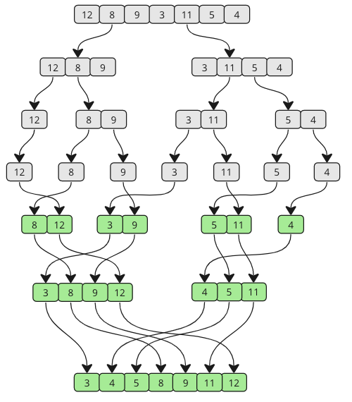
The Merge Sort algorithm is a divide-and-conquer algorithm that sorts an array by first breaking it down into smaller arrays, and then building the array back together the correct way so that it is sorted.

1. Divide the unsorted array into two sub-arrays, half the size of the original.
2. Continue to divide the sub-arrays as long as the current piece of the array has more than one element.
3. Merge two sub-arrays together by always putting the lowest value first.
4. Keep merging until there are no sub-arrays left.

Sorting of an arraySorting of a linked list

def sortList(arr):
    step = 1  # Starting with sub-arrays of length 1
    length = len(arr)

    while step < length:
        for i in range(0, length, 2 * step):
            left = arr[i:i + step]
            right = arr[i + step:i + 2 * step]

            merged = merge(left, right)

            # Place the merged array back into the original array
            for j, val in enumerate(merged):
                arr[i + j] = val

        step *= 2  # Double the sub-array length for the next iteration

    return arr

def merge(left, right):
    result = []
    i = j = 0

    while i < len(left) and j < len(right):
        if left[i] < right[j]:
            result.append(left[i])
            i += 1
        else:
            result.append(right[j])
            j += 1

    result.extend(left[i:])
    result.extend(right[j:])

    return result

def sortList(head: Optional[ListNode]) -> Optional[ListNode]:
    if not head or not head.next:
        return head
    slow, fast = head, head
    prev = None
    while fast and fast.next:
        prev = slow
        slow = slow.next
        fast = fast.next.next
    prev.next = None
    left = sortList(head)
    right = sortList(slow)
    return merge(left, right)

def merge(l1, l2):
    dummy = ListNode(0)
    cur = dummy
    while l1 and l2:
        if l1.val < l2.val:
            cur.next = l1
            l1 = l1.next
        else:
            cur.next = l2
            l2 = l2.next
        cur = cur.next
    if l1: cur.next = l1
    if l2: cur.next = l2
    return dummy.next

Selection

Quickselect

TODO